GRASS can execute a perfectly valid raster expression and still answer a different spatial question from the one its operator intended. The expression may name the right elevation map and use the right threshold, yet its output can cover the wrong extent, land on the wrong cell grid, or silently exclude a study area. That is not randomness. It is an architectural clue: in GRASS, the command string is only part of the program.
The rest lives in an analysis environment. A project fixes the coordinate reference system. A mapset supplies a write namespace and a search path. A computational region supplies the working extent, resolution, and alignment. An optional raster mask changes which input cells participate. Most raster modules consult that state without requiring it to be repeated on every command line.[2][4][5][7]
Calling this state a collection of defaults undersells it. It is closer to an execution contract for space. The contract makes long chains of geoprocessing modules composable: once the working grid is deliberate, successive outputs line up without every module negotiating a new one. It also creates a reproducibility obligation. Saving only the final r.mapcalc expression is like saving a database query without recording which database or schema resolved its names.
GRASS has carried versions of this model through an unusually long life. Work began at the U.S. Army's Construction Engineering Research Laboratory in 1982, and stewardship later moved into an international free-software community.[1] The contemporary interfaces are very different from those early systems, but the durable idea is still visible: analysis happens inside a prepared geographic workspace, not against a loose pile of unrelated files.
A project fixes geography; a mapset fixes where work lands
A GRASS project contains data in one coordinate reference system. Inside it, mapsets divide the work into subprojects or working environments. Every project has a mapset named PERMANENT, conventionally used for shared base data and the project's default region. Analysts can create separate mapsets for people, scenarios, or batch jobs while reading the same baseline maps.[2][3]
The current mapset is a session-relative write boundary. A module can create, modify, or remove maps there, while other permitted mapsets are read through a search path. This is namespace discipline, not a security sandbox and not a promise that PERMANENT is immutable: a user who makes another mapset current and has permission to it can write there. The architectural benefit is narrower and useful—ordinary work has one obvious destination.[2][3]
Reading is more subtle. An input named elevation resolves to the first matching map on the search path, with the current mapset first and PERMANENT included by default. elevation@PERMANENT names one mapset explicitly. That difference can change results without changing the mathematical expression. If a scratch mapset contains its own elevation, a bare name can shadow the shared baseline; if two mapsets save different search-path orders, the same bare name can bind to different data.[2]
This is why mapsets work well for parallel scenarios but do not make provenance automatic. Give each run its own current mapset and outputs will not trample one another. Qualify important inputs with @mapset, however, or the convenience of shared names becomes an undeclared dependency.
The computational region is an implicit argument
Each mapset has its own current computational region, normally persisted in a file named WIND. The PERMANENT mapset also holds DEFAULT_WIND, which supplies a project's default and the starting region for new mapsets. Changing the current region does not crop or rewrite stored maps. It changes the grid on which subsequent region-aware work is evaluated.[3][4]
That grid contains north, south, east, and west bounds, plus row and column resolution; three-dimensional rasters add a vertical dimension. Most raster and display modules honor it, while vector modules generally do not, and import, projection, and explicit resampling tools are among the exceptions. g.region can copy a raster's grid, target a named extent, set rows or resolution, align boundaries, save a named region, or print the active settings.[4][5]
The resolution is not cosmetic. Consider a session in a metre-based projected coordinate system over a nominal 10-kilometre-square study area. At 10-metre cells, it contains about one million cells. At 1 metre, it contains about 100 million—100 times as many values before an algorithm's own overhead is considered. A one-character change to res can therefore alter both analytical meaning and computational cost. Boundary alignment may adjust the exact row count, but the scale change remains.
A small, inspectable setup might begin like this inside a known GRASS session:
g.region -a raster=elevation@PERMANENT res=10
g.region -p format=json > run-region.json
r.mapcalc "high_ground = if(elevation@PERMANENT >= 500, 1, null())"
The first line makes the intended source extent and 10-metre grid explicit, with boundaries aligned to the resolution. The second serializes the effective region in machine-readable form. The third writes a new raster to the current mapset and records its formula in the result's title and history.[4][6] That JSON file is valuable evidence, but it is not a complete run manifest: it says nothing about an active mask, map identities, software build, or process-level overrides.
Raster inputs meet on the region's grid
By default, GRASS reads raster inputs through the current region. An input with a different extent is cropped or padded with NULL cells; one with a different resolution or alignment is resampled on the fly to the working grid using nearest-neighbour selection. Raster outputs take the current region's bounds and resolution. The original input is not rewritten.[5]
This behavior is powerful because raster algebra can combine maps without first manufacturing a matched copy of every source. It is also opinionated. Nearest-neighbour selection preserves categories well, but it is not automatically the right scientific choice for a continuous surface. When interpolation or aggregation matters, the workflow should use an explicit resampling module and document the method rather than treating automatic grid matching as neutral.[5]
r.mapcalc makes the composition especially clear. It evaluates cell expressions, follows the mapset search path for unqualified names, propagates NULL according to its operators, and creates its named output in the current mapset. Its default computation region is the current one, though current releases also offer union and intersect modes that derive a temporary region from input maps without changing the stored mapset region.[6]
The recorded formula is therefore necessary provenance, not sufficient provenance. Two result histories can show the same expression while their raster headers reveal different grids. Two identical expressions and grids can still have read different shadowed inputs. The important unit of review is not just “what equation ran?” but “what equation ran over which lattice, resolving which maps?”
A mask is a second, quieter spatial input
The computational region describes a rectangle. A raster mask describes which cells inside that rectangle count. When a mask is active, data outside it are treated as NULL as existing raster inputs are read. When given a raster input, r.mask normally creates a reclass raster named MASK; that mask remains active until it is removed or renamed, and the GRASS_MASK environment variable can select a different mask name.[7]
There is a particularly sharp edge around zero. With its default category selection, r.mask raster=input converts every non-NULL input value, including zero, to 1. If zero was meant to mean “outside,” that invocation includes it. By contrast, a raster created directly as the effective MASK behaves like a Boolean mask: zero and NULL are excluded, while nonzero integer values are included. The two creation paths look similar at a glance and do not mean the same thing.[7]
Masks also act on reads, not as a universal stencil over every write. An expression that reads elevation sees masked-out cells as NULL. A constant expression need not read a raster at all, so assuming that every output is clipped merely because a mask is active is unsafe.[6][7]
This ambient behavior is excellent for a session in which dozens of operations must use one watershed or administrative boundary. Set the mask once and the analyst avoids repeating a clipping operand. In an unattended pipeline, the same persistence can become technical debt. A forgotten mask can generate clean-looking, internally consistent, incomplete outputs. A defensible run should declare whether the mask is absent, name exactly which raster supplies it, and record how that raster was built.
The reproducibility unit is larger than a command
The architecture suggests a concrete operating pattern. Start in a named project and a fresh, uniquely named mapset. Fully qualify baseline inputs. Set and export the computational region before analysis. Establish or remove the mask deliberately rather than inheriting whatever a previous interactive session left behind. Record the GRASS release, module parameters, input checksums or stable dataset identifiers, search path, region JSON, and mask status beside the output. Inspect the output header and history before export.
That may sound heavier than opening a GeoTIFF and calling a function. It is heavier. An independent 2025 review of digital urban-planning tools reached a similar adoption boundary from the user side: it singled out GRASS for the depth of its analytical functions while also identifying a steep professional learning curve.[9] Teams that need only a few stateless transformations may reasonably prefer a smaller library. Teams building repeatable hydrology, terrain, imagery, or land-change pipelines can benefit from a workspace that makes one CRS, a deliberately selected working grid, and separate run namespaces durable concepts.
GRASS 8.5.0 shows the project trying to expose that mature engine through more contemporary automation. Released in May 2026, it added a higher-level grass.tools Python API, more JSON outputs, direct array-oriented raster exchange, and parallel execution improvements including work on r.mapcalc.[8] Those interfaces reduce ceremony; they do not abolish the spatial contract. A Python call still needs to know which project, mapset, region, and mask give it meaning.
That is the useful way to read GRASS's architecture. The computational region is not merely the rectangle currently visible on a screen. The mapset is not merely a folder. Together with name resolution and masking, they are inputs to the computation—inputs made persistent so a family of tools can agree. Once a workflow records them with the same care as its formulas, GRASS's ambient state stops being a trap and becomes what it was designed to be: a shared definition of the geographic question.
Sources
- GRASS project, “History of GRASS” — CERL origins, transition to community stewardship, and open-source milestones.
- GRASS 8.5 documentation, “GRASS projects” — one-CRS projects, mapsets, current-mapset writes, search paths, qualified names, and temporary workspaces.
- GRASS 8.5 documentation, “GRASS database” — project/mapset storage hierarchy and the
WINDandDEFAULT_WINDregion files. - GRASS 8.5 manual, “g.region” — computational-region extent, resolution, alignment, persistence, scope, and JSON output.
- GRASS 8.5 manual, “Raster data processing in GRASS” — region-controlled outputs, input cropping, padding, rescaling, NULL behavior, and exceptions.
- GRASS 8.5 manual, “r.mapcalc” — raster expressions, mapset name resolution, computation-region modes, output location, and formula history.
- GRASS 8.5 manual, “r.mask” — persistent raster masking, creation paths, zero and NULL semantics, removal, and named masks.
- GRASS project, “GRASS 8.5.0 released” — May 2026 release context,
grass.tools, JSON interfaces, array exchange, and parallel-processing changes. - Samuel Hanan and Neil Carhart, “A review of urban planning tools for empowering public participation,” Frontiers of Urban and Rural Planning — independent comparison of GRASS's analytical depth and adoption learning curve.
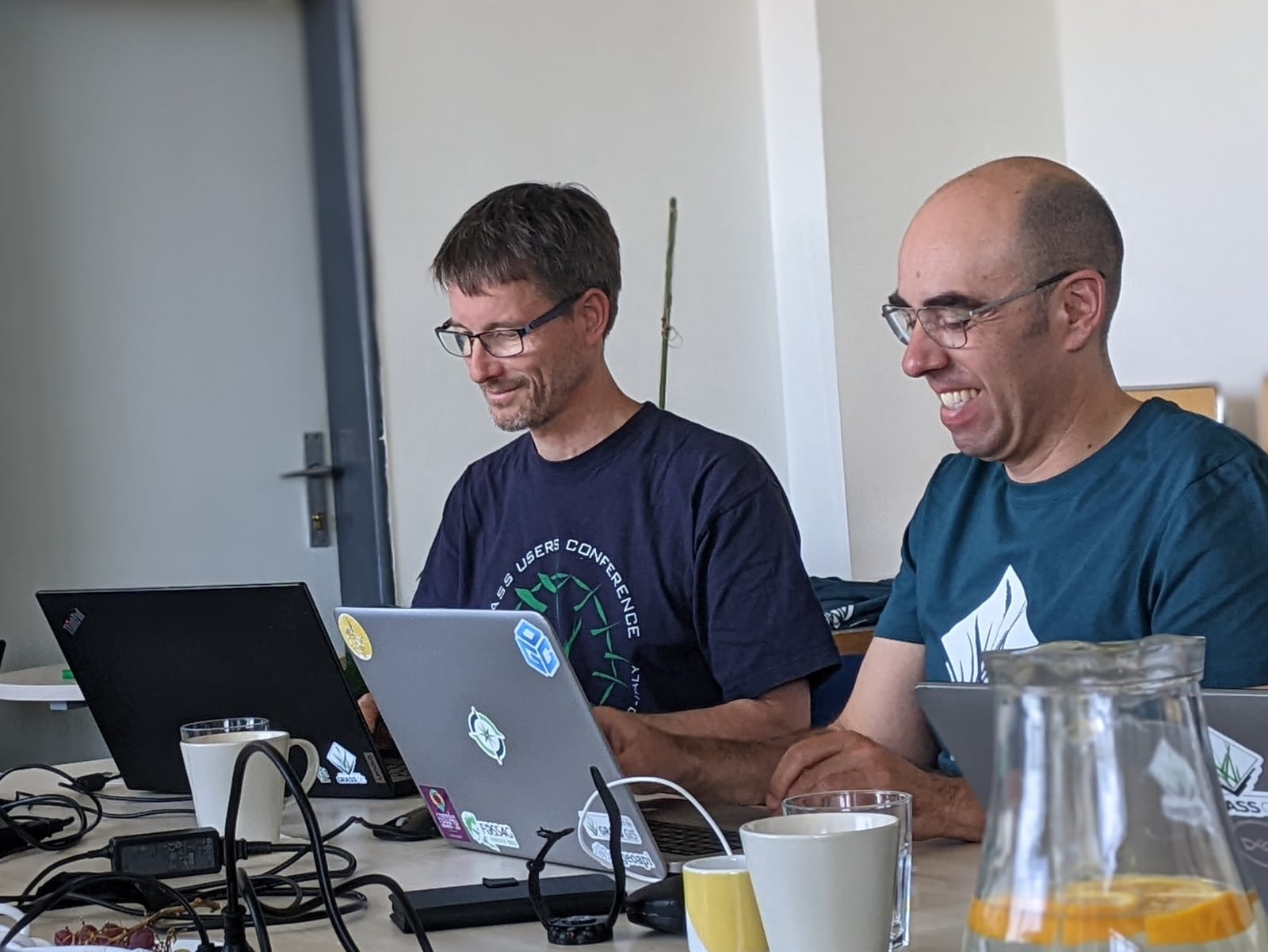
- GRASS project, “GRASS Community Meeting Prague 2023” — event record and source gallery for the cover photograph.