A simulated waveform looks continuous. The open-source circuit simulator ngspice builds it from discrete calculations, starting with a description of the circuit and ending with saved results. Its architecture is easiest to understand by following three decisions: what is connected, how the circuit begins, and whether the next time step is acceptable.[1][2][4]

Those decisions matter when a pulse develops an unexpected shoulder, an amplifier refuses to settle, or a run ends with a time-step error. Each offers somewhere to investigate before changing a setting and trying again.

The drawing becomes a set of connections

Ngspice's own account of its internals begins with a netlist. Before solving anything, the program processes such features as subcircuits and parameters, constructs its circuit representation, and assembles a matrix. Simulation and output processing follow. A schematic editor can supply the description, but the solver works on the resulting mathematical circuit.[1]

The difference is visible in a tiny fragment: R1 in out 1k describes a resistor between two named nodes. It says nothing about where the resistor sits on a drawing. Node 0 supplies the ground reference. These names and connections are part of the executable input, rather than labels added to a finished picture.[2]

KiCad provides an instructive view from outside the ngspice project. Its simulator documentation warns that a symbol's pin numbers can differ from the simulation model's terminal order. A diode or operational amplifier may need explicit mapping in the Pin Assignments tab. The symbol can look familiar while the model is connected incorrectly.[3]

This gives an apparently numerical problem a possible upstream cause. Before interpreting an unusual waveform, establish what the solver was actually asked to connect. In that sense, inspecting the model assignment belongs alongside inspecting the wiring.

A transient needs somewhere to begin

Ordinarily, ngspice computes an initial operating point before a transient analysis. Independent sources take their time-zero values; capacitors are treated as open circuits and inductors as shorts for that calculation. Nonlinear device equations are solved iteratively. The optional uic keyword bypasses this operating-point calculation and uses specified initial conditions instead.[2]

For an ideal resistor-capacitor circuit on a constant supply, the settled starting point already has the capacitor charged. Studying power-on behavior requires describing the input change or an appropriate initial state.

Solving the equations is only the first test

Holger Vogt's account of time-step control describes two tests. Failed matrix convergence sends ngspice back with a shorter interval. After convergence, it still estimates local truncation error—the error from advancing through a finite interval. An excessive estimate can reject the step too.[4]

Convergence concerns the solution at the proposed time; the error check concerns how accurately the integration reached it. Passing one does not guarantee passing both. Repeated reductions can eventually end with “Timestep too small” at the lower limit.[4]

The .tran directive exposes a maximum step through tmax. For example, .tran 10u 5m 0 1u requests a run ending at 5 milliseconds, with a 1-microsecond maximum step. That maximum is a ceiling; the internal intervals may be smaller.[2][4]

An engineering consequence is that a time-step failure deserves diagnosis. Changing a numerical setting may help, but the setting alone cannot tell you whether the starting conditions, connections, or component models describe a plausible experiment.

Keep the experiment with the result

Ngspice's control language makes this chain repeatable. Commands between .control and .endc can run analyses, change component values, repeat a sweep, and write results to a file. The project's tutorial demonstrates altering a supply voltage across successive runs. It also explains that a ngspice “plot” is a group of data vectors, even when no graph is displayed.[5]

This separation is useful: computation does not depend on someone keeping a plotting window open. A sequence can preserve both the changed input and the resulting vectors. The tutorial's destroy command also makes storage visible as a resource constraint; accumulating every run's vectors consumes memory.[5]

For a small electronics team, my practical inference is to retain the netlist, model files, simulator version, and control commands together. That gives a colleague a repeatable experiment to inspect when a component substitution changes the result. A screenshot alone leaves too many of those choices unstated.

The bench supplies a different kind of evidence

Numerical acceptance still applies to the supplied model. In an independent explanation of SPICE limitations, Analog Devices applications engineer John Ardizzoni notes that amplifier macromodels omit characteristics to manage complexity, development effort, and simulation speed. When an Analog Devices model conflicts with its datasheet, he advises trusting the measured datasheet information. He also emphasizes physical prototyping, particularly where board construction affects high-speed behavior.[6]

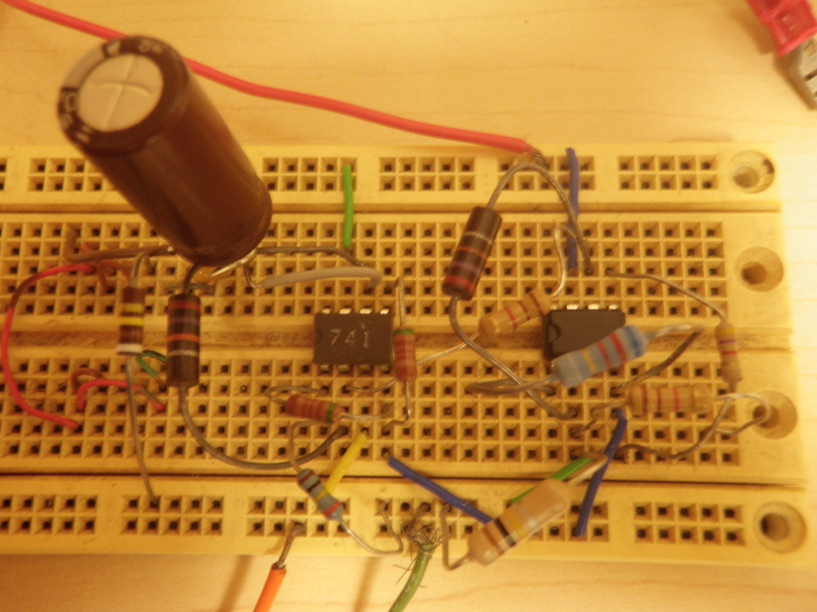
That is a separate boundary from time-step accuracy. More careful integration cannot introduce a physical effect absent from the model. Nor can a correct model assignment establish that the circuit on the bench has been wired as intended.

Ngspice makes the computational experiment inspectable at several levels: connections, starting conditions, numerical progression, and saved output. Its architecture helps locate a disagreement. The next useful action depends on which level failed: correct a terminal mapping, reconsider the initial state, investigate a rejected step, or measure the physical circuit. A convincing waveform becomes more valuable when the path that produced it remains available for scrutiny.

Sources

1. Ngspice project, “Documentation,” section “Ngspice Internals”—netlist processing, circuit construction, matrix assembly, simulation, and output.
2. Ngspice User's Manual, version 47, chapters 2 and 11—netlists, initial conditions, and transient parameters.
3. KiCad 9.0 Schematic Editor documentation, “Simulator,” especially “Pin Assignment”—an independent integration reference explaining symbol-to-model terminal mapping.
4. H. Vogt, “Time step control in ngspice” (November 23, 2025), DOCX—step acceptance and rejection.
5. Ngspice project, “Tutorial: ngspice control language”—scripted runs, supply sweeps, result vectors, file output, and releasing plot memory.
6. John Ardizzoni, “Which carries more weight a datasheet or SPICE macromodel?”, Analog Devices, Rarely Asked Questions, issue 47—independent engineering commentary on model limits and physical verification.
7. Jstapko, “2 stage amplifier with op amps” (November 9, 2012), Wikimedia Commons—original breadboard photograph, description, and attribution.